Graphic/Numeric Maps

The Graphic/Numeric Map Layer allows users to display global maps in the Viewing Window. These maps usually serve as the basis of the Viewing Window, with other layers (such as the ROI Layer, Groundtrack Layer, etc) displaying on top of them. The Graphic/Numeric Map Layer is a simplified version of the Advanced/Custom Map Layer with interfaces that will be familiar to long-time JMARS users. 

 Display a Graphic Map

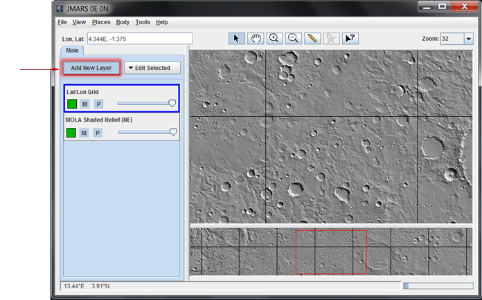
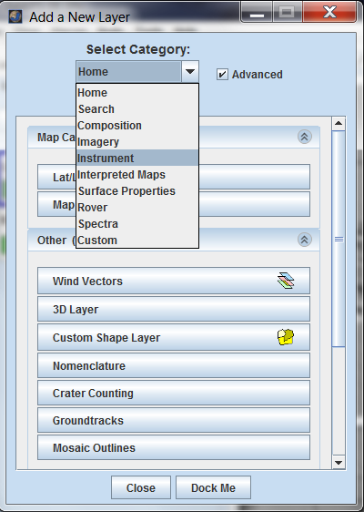
1. Open the Map: Choose "Add New Layer" and then click the drop-down tab and select "Instrument". Then click the "Subcategories" tab and select the data you would like. Follow the menu structure to the map you want to load and choose "View Graphic Data". Example is given below.
   

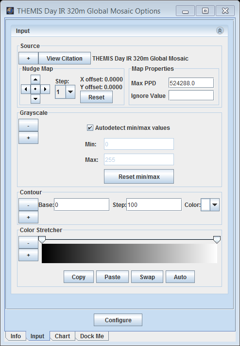
2. Edit Basic Map Settings: In the Layer Manager, click on the tab of the map you would like to edit. This will display the map's focus panel, which contains all the basic map settings users can modify.

1. Nudge the Map: If users don't believe the graphic map loaded in the correct location, they can "nudge" it in any direction using the arrow controls in the focus panel. The default step size is one pixel, which can be changed using the drop-down menu.
2. Map Resolution: The default (highest) resolution of a map is displayed in the "Max PPD" section of the "Map Properties" box. If users want to reduce the resolution of the map (ie: to match the resolution of another dataset), they can do so by changing this value.
3. Ignore Value: Many of the global maps have gaps where the given instrument did not collect good quality data. If you want these areas to appear transparent in JMARS, set the ignore value to the value of the blank pixels in the gaps.
   • The blank pixels in all the default JMARS maps are set to a value of "0". The default ignore value is also set to zero, so these areas will appear transparent by default.

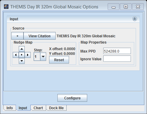
3. Edit Advanced Map Settings: Advanced users can access additional map settings by clicking the "+" button in the "Source" box of the focus panel and then selecting which category of settings they wish to modify. Depending on the type of map being displayed, some categories may not have meaning and will therefore not be displayed. The possible categories are:
   1. Gray Scale: The grey scale being used to colorize a graphical map can be adjusted by changing the min and max values of the gray scale.
   2. Color Stretcher: If users want to apply a different color scale (ie: a red scale or a spectrum scale) to the dataset, they can right-click on either the left or right tabs of the color spectrum, choose "Set Tab Color" and then choose from the available color options.
   3. Contour: User can add contour lines to most maps. For more information, please see the "Creating Contour Maps" section below.

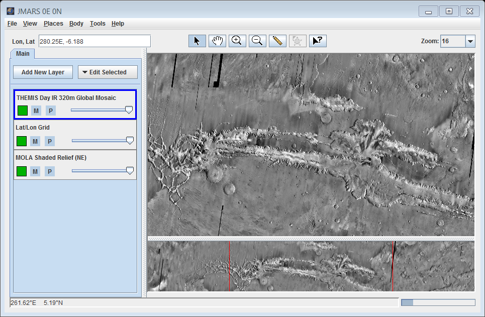
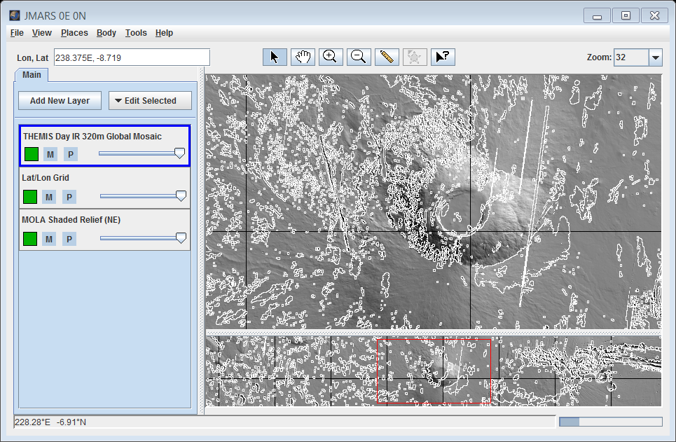
• After applying the above setting on Themis Day IR Global Mosiac the map looks as shown below.

4. Edit Map Configurations: Very advanced users can manipulate all of the settings associated with the maps by using the "Configure" button at the bottom of the focus panel.
   • Clicking on the "Configure" button will open up the settings window associated with the Advanced/Custom Map Layer and allows users to edit the configuration of the map. 

Plot Values from a Numeric Map

1. Open the Map: Choose "Add New Layer" and then Click the Home drop-down tab and select "Instrument". Select the numeric data you would like.
   • Loading a numeric map will not cause any changes in the Viewing Window since it has no graphic data. All the numeric data exists in the background and is represented by a new tab in the Layer Manager. (Think of it as an invisible map.)
   • Some maps, such as the TES Mineral Maps, contain both graphic and numeric data. Users can choose to Plot and View Graphic data in the Advanced/Custom Map Layer if they want to load both the graphic and numeric datasets.

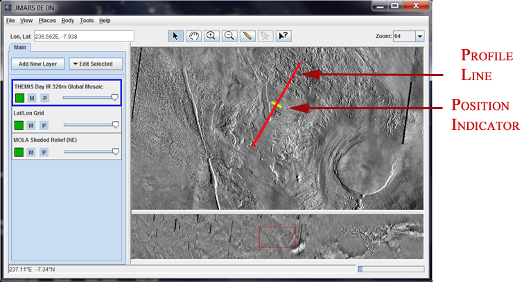
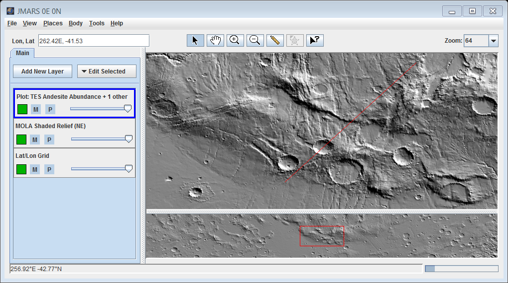
2. Draw a Profile Line: In the Viewing Window, click to start a profile line and then double-click to end the profile line. The data along that line will be plotted in the focus panel under the "Chart" tab.
   • Users can create non-linear profile lines by clicking to start the line, then single-clicking to add intermediate points and finally double-clicking to end the line.

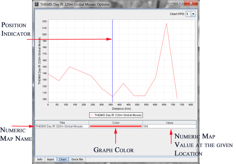
3. Retrieving Specific Data Points: To read the exact values of the graph at a given point, move the yellow placemarker on the profile line to the desired location. In the focus panel chart, the x-axis value is the position along the profile line and the y-axis value is obtained from the selected numeric map at that position. The exact y-axis value is displayed in the "Value" column under the plot.

4. Zooming in on the Plotting Window: Left-click and dragging in the focus panel's plot window will create a box. When users release the left-click button the plotting window will zoom in on the selected area. Users can also right-click and choose to either zoom in or out.

5. Using the "Configure" Button: Clicking on the "Configure" button will open up the settings window associated with the Advanced/Custom Map Layer and give users full control over all map settings. 

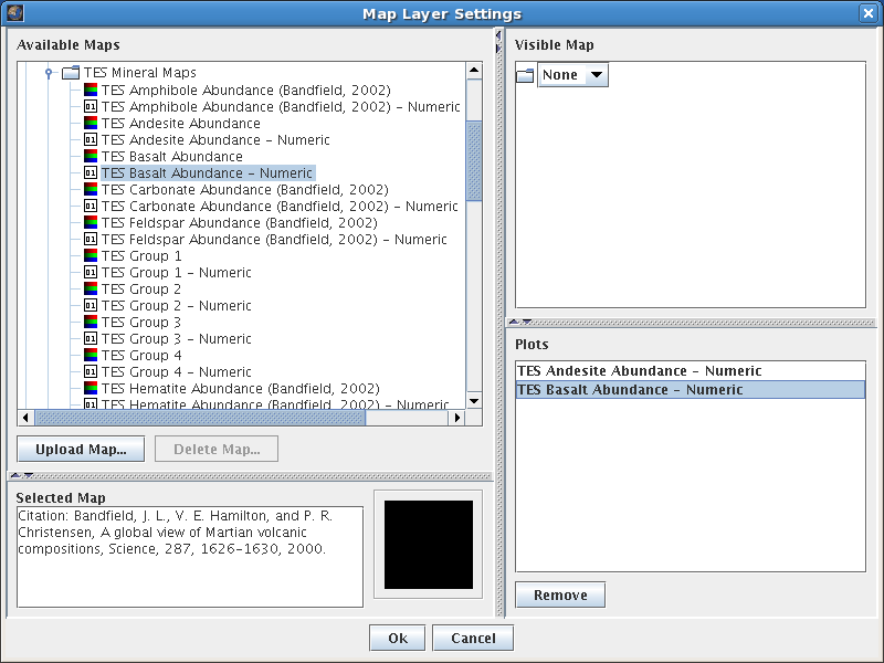
Graph Values from Multiple Numeric Maps

1. Open a Numeric Map: Load a numeric map using either the Graphic/Numeric Map Layer or the Advanced/Custom Map Layer

2. Open the Configuration Window: In the Layer Manager, click on the tab of the first numeric map, then click on the "Configuration" button at the bottom. The Advanced/Custom Maps settings window will appear.
   • The name of the numeric map that has already been loaded will appear in the "Plots" section.

3. Load Additional Numeric Maps: Under the "Available Maps" section, select another numeric map by clicking on "Mars Spaceflight Facility MapServer" and following the menus to the desired map. Then left-click and drag the numeric map name into the "Plots" section.
   • Numeric maps are labeled with a "01" icon.
   • The maps listed under "Mars Spaceflight Facility MapServer" are organized in the same menu structure used by the "Add New Layer" button in the Layer Manager.

4. View a Plot of the Numeric Data: Draw a profile line in the Viewing Window and the values from all loaded numeric datasets will be plotted in the focus panel.

Creating Contour Maps

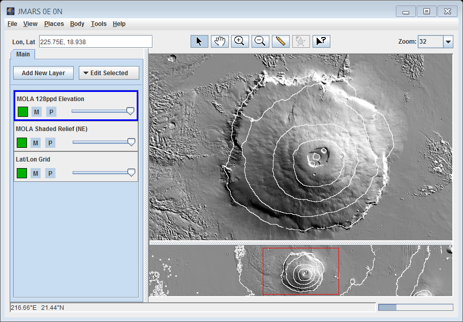
1. Create a MOLA Elevation Contour Map
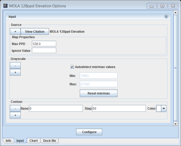
   1. Open the Numeric MOLA Map: In the Layer Manager, choose Add New Layer -> Instrument -> MOLA -> MOLA 128ppd Numeric Elevation. Then double click the newly added Mola map inside the layer manager and select the "Input" tab at the bottom.

2. Edit Contour Map Properties: Under "Greyscale" there is a minus and plus button. Click the plus button -> "Contour". Here, the user can specify the base elevation, the step size and the color of the contour lines.

2. Contour Nunmeric Data other than MOLA Elevation
   1. Other datasets can be contoured as long as it is a numeric dataset.

3. Contour Graphic Data

Contour lines can also be added to graphic data, but the lines will only represent changes in the pixel values of the image.

1. Open a Graphic Map: In the Layer Manager, go to "Add New Layer" and open the graphic map you would like to add contour lines to.
2. Change Map Settings: Click on the tab for the graphic map in the Layer Manager. In the focus panel, click on the "Input" tab. On the "Input" screen, click on the "+" button in the "Source" section and choose "Contour" from the drop-down menu.
   • A contour map will be created using the default values. Users can edit these values in the "Contour" section of the focus panel, which will cause the contour map to be re-drawn with the given specifications.

An introduction to JMARS Video Tutorial: Numeric Profiles

---

Related Pages

• Tutorial #1: Viewing THEMIS VIS Coverage
• Tutorial #2: Displaying the Main View in 3D
• Tutorial #3: Finding THEMIS Observation Opportunities